Partial Discharge Testing of HV Assets: How Often Should We Test?

Partial discharge testing, an established condition monitoring test, plays a pivotal role in determining HV asset health. When embarking on a PD testing programme, the challenge lies in tailoring a testing schedule that yields high-quality data and identifies faults promptly, allowing time for intervention to prevent failure.

Through studying the P-F curve and how that applies to HV switchgear, this article explores how optimal testing frequency may be determined, examining various P-F curve scenarios, and evaluating the benefits and drawbacks of periodic testing versus permanent monitoring.

Partial Discharge Variants

PD can be classified into 3 main types, Internal, Surface and Corona.

Internal PD: An Invisible Threat

Internal PD silently occurs giving no external warning such as sound, smell or any visual indication of a problem. The first indication of problems may be drastic failures, like the catastrophic cable box failures of the past.

Prior to the UK electricity industry’s privatisation, EA Technology, then known as the Electricity Council Research Centre, researched the detection of such PD activities.

A significant breakthrough was Dr. John Reeves’ identification of Transient Earth Voltages (TEVs) due to PD, leading to the creation of the first TEV instruments.

Internal void discharges were the main cause of unanticipated equipment failure and these often slow evolving defects. TEV testing every 2 years and a week-long monitoring of primary switchboards every 4 years, was widely adopted.

Surface PD: A More Visible Concern

In the late ‘70s and ‘80s, switchgear insulation underwent significant changes: air-insulated chambers supplanted bitumen, and porcelain gave way to cast resin. The industry also broadly adopted dry terminations. Yet, these shifts, combined with overlooked design and installation details, led to a rise in failure rates due to surface PD.

Surface PD differs from internal voids by emitting lower amplitude but more frequent pulses. If you hear crackling or detect ozone odours, it suggests advanced insulation degradation.

The real challenge was early detection. Research pinpointed ultrasonic testing as an essential complementary technique to TEV for these types of defects.

Environmental conditions, particularly humidity, greatly affect surface PD. In chambers with limited ventilation, PD by-products like nitrous oxides combine with moisture, forming nitric acid.

This acid accelerates insulation deterioration and amplifies PD sites, leading to faster failures. Hence, the industry typically shifted from biennial to annual inspections.

Corona PD

Corona PD, while not inherently harmful in outdoor switchyards, can initiate surface PD if left unchecked in enclosed chambers, leading to the onset of surface PD.

The P-F Curve: A Guidepost

The P-to-F Curve represents the progression of equipment failure over time. It’s commonly used in predictive maintenance to understand and illustrate the stages from a potential failure point (P) to a functional failure point (F).

• P (Potential Failure): The point at which a failure first becomes detectable but the equipment is still functioning properly.
• Condition Monitoring Phase: Between P and F, condition monitoring tools can detect worsening conditions, allowing for interventions before a functional failure.

The curve underscores the importance of early detection, allowing maintenance personnel to act during the window between potential and functional failure, thus preventing unexpected outages and associated costs.

When dealing with HV switchgear and the multiple variables in play, the P-to-F curve becomes more complex. Each type of failure or variable may have its own distinct P-to-F curve, which can vary in length and shape.

Factors which will influence the rate of degradation within the insultation, either increasing or decreasing the P-F interval include:

• Type of partial discharge
• Type of HV asset
• Discharge amplitude
• Insulation type 
• Environmental conditions
• Physical position of discharge

Given these factors, predicting the precise duration of the P-F interval is challenging. It can range from weeks to months or years, depending on the specific defect.

The variability in the P-F interval can make it challenging to devise an optimum testing regimen. To maximize the likelihood of early defect detection, it’s crucial to design the testing strategy around defects with shorter P-F intervals rather than those with longer ones. However, resource and economic constraints might not always make this approach feasible.

Case Studies: Practical Insights

Case 1: Yearly Testing

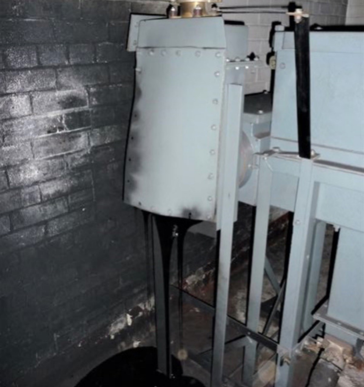
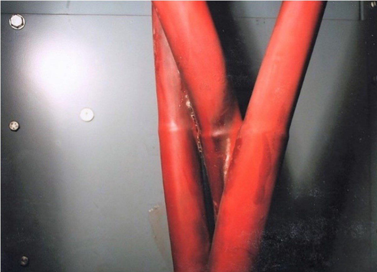
A network operator, conducting annual PD tests, detected an ultrasonic PD source in a cable box after 5 years of testing. Unfortunately, the asset failed in service within the year prior to the next scheduled maintenance or PD test, leading to significant disruptions.

The defect site of this failure was found to be in the crutch of the original 11kV PILC cables that were reused when the RMU was replaced. The defect site was likely introduced during the commissioning of the new RMU.

Figure 5 shows a timeline of the RMU and testing.

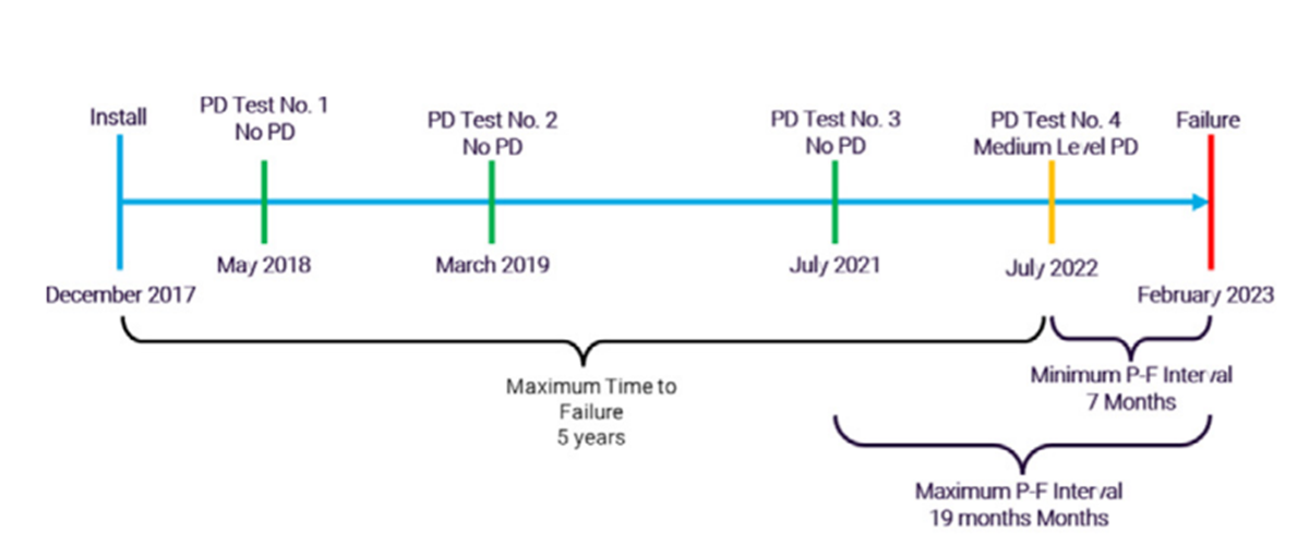
Given the assumption that the defect originated at the time of commissioning, time to failure was 5 years. For this specific defect, the P-F interval ranges from a minimum of 7 months to a maximum of 19 months

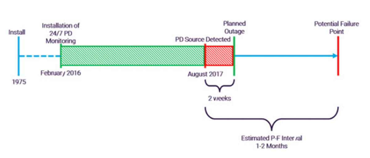
Case 2: Permanent Monitoring

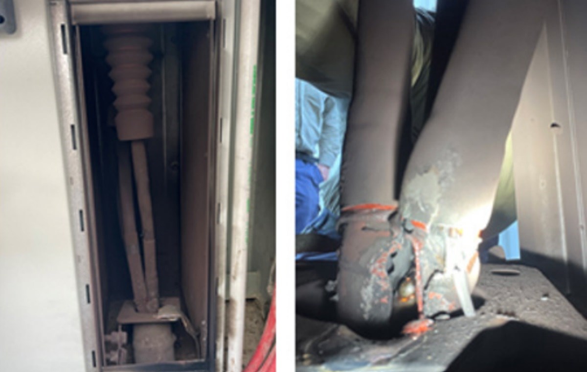
Due to the critical nature of an aged 11kV switchboard, 24/7 PD monitoring was initiated to mitigate risk. Within 18 months, an emerging failure was detected on a voltage transformer, with data showing the rise in PD activity from zero to a high level in a matter of minutes.

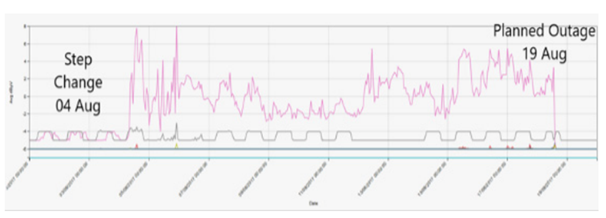
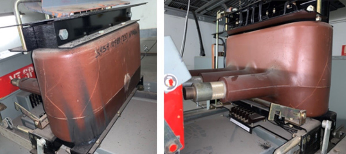
An outage was scheduled to inspect the VT. The assessment revealed significant damage, indicating the component was nearing failure. Thanks to timely intervention, no customers faced any disruption or interruption to supply, and no other components on the switchboard were negatively impacted.

The exact P-F interval is unknown due to intervention before failure due to the early warning. However, based on the amount of damage to the insulation after two weeks of operation, the estimated P-F interval is 1-2 months.

The full timeline for this event is shown below in Figure 8.

Designing a Test Regime

RCM theory states that the testing interval should be approximately half of the P-F interval for the failure of an asset. However, this is difficult to apply to high voltage assets, due to the variability of the P-F interval and its affecting factors.

Case Study 1 demonstrated that an annual test can identify emerging PD defects but may not efficiently track their progression if the P-F interval is relatively short.

While more frequent testing could potentially catch these issues earlier, the practicality and costs associated with such measures can be limiting.

In contrast, Case Study 2 pointed to a defect with a notably brief P-F interval of 1-2 months. An annual test presents merely a 1 in 6 chance of detecting this defect after its onset and before failure. Even a 6-month interval only doubles this chance to 1 in 3.

Given the switchboard’s criticality, the installed 24/7 monitoring was invaluable, providing the operator ample time to take preventative measures.

These case studies suggest a strategy of tailoring testing intervals to asset risk and criticality

Summary

Considering the P-F curve is beneficial for devising effective testing regimes. Yet, understanding the multifaceted variables influencing the P-F interval for high-voltage assets is essential. This interval can vary extensively, from weeks to years.

For optimal test design, one should account for the shortest plausible P-F interval within the network. By narrowing the testing interval, we can enhance our chances of identifying defects closer to their onset and provide time to act before full-scale failure occurs.

As a result, permanent PD monitoring emerges as the most effective approach to detect defects at their inception, giving operators the maximum response window and reducing the potential risks of HV failure.

For expansive HV networks, while continuous monitoring significantly reduces the risk of HV failure, a balanced approach combining periodic testing with such monitoring often proves most effective. A risk evaluation of assets will determine where more frequent testing or permanent monitoring is most essential.

Contact us to learn more about the most suitable monitoring regimes for your asset types.